Overview
In this style tutorial, we'll be setting up the same style that is used in the
batch rating sample from scratch. If you haven't used the batch rating sample yet, please
try it first.
We're going to create a style that is used to rate packages for shipment. We'll provide more than the required information so we can get more accurate rates and for ease of use. We'll record the cost to ship the package, information about when it will arrive, and any potential errors.
1. Decide what information to provide to UPS
There is a minimum amount of information that must be provided for each transaction. For rating, we have to provide the destination state and zip code, the service to use, and the package weight. You can see the minimum requirements for each transaction here:
Minimum Fields to Map.
We are also going to provide some additional information to make the rates more accurate and to help people use the Excel file more easily. These extra details include the contact name and company name, the street address, and the country in case we need to rate anything international.
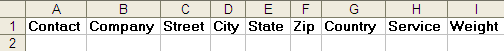
In Excel, create a column heading for each of the following:
-
Contact
-
Company
-
Street
-
City
-
State
-
Zip
-
Country
-
Service
-
Weight
2. Decide what information we would like to record
We can get a good amount of information back from each of the transaction types. We're actually going to record everything we can so that we end up with as much information as possible. You can see the information available for each transaction here:
Batch Data Returned.
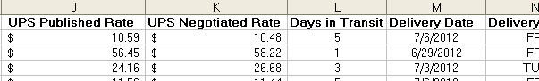
The following information is available when we rate a package. In Excel, create a column heading for each one:
NOTE: You should always record the error in case anything goes wrong. The details noted in the error will help you to resolve any issues.
3. Create a new style
Now we'll create the style so OzLINK knows what transaction to use and what the columns in the spreadsheet actually mean.
A. Click on the Styles button in Excel.
Microsoft Office 2003 or earlier:
The OzLINK buttons will be in your main toolbar, and look like this:
Microsoft Office 2007 or later:
Click on the Add-Ins tab to find the OzLINK buttons:
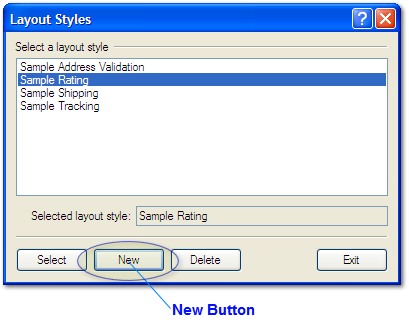
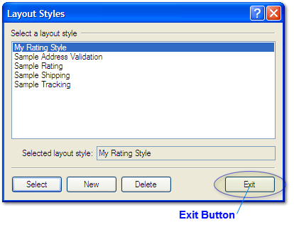
B. In the Layout Styles dialog box that opens, click the New button.
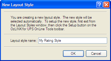
C. Enter "My Rating Style" for the new style name, then click OK.
D. Your new style is now created, but not yet configured. It should be listed in your style list. Notice that your new style is also the active style, indicated by the "Selected layout style: " box. Click Exit on the Layout Styles dialog box that appears.
4. Set up the transaction and workflow options
In this step we'll configure the transaction and workflow settings for our new style.
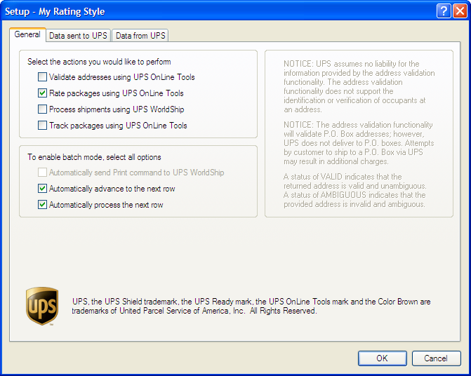
B. In the Setup window that appears, choose
Rate packages using UPS Online Tools for our action. If you'd like more details about each type of action, see:
Batch Actions and Workflow.
C. In the batch mode section, choose
Automatically advance to the next row and
Automatically process the next row. If you'd like more details about the workflow options, see:
Batch Actions and Workflow.
Your setup screen should now look like this:
5. Map the information you're sending to UPS
In this step we'll tell OzLINK what kind of information is in each of the Excel columns. We'll work on the information that is being sent over to UPS for the rating task, then in step 6 we'll work on telling OzLINK which columns should store the reply. The process of matching your Excel columns to the appropriate information is called mapping the data.
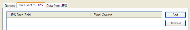
A. Click on the Data sent to UPS tab. Right now there is nothing in the list - we'll be adding an entry for each Excel column.
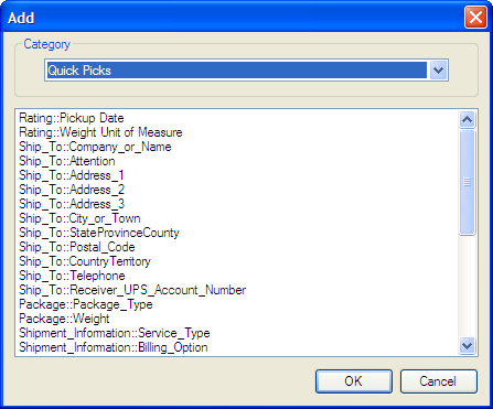
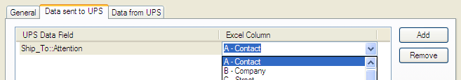
B. Click the Add button to add a new entry. The screen below will appear. The first column in our Excel sheet is Contact, so choose Ship_To::Attention, then click OK.
C. Ship_To::Attention will now be listed in the UPS Data Field section of the window. Next to it, in the Excel Column, click on the dropdown list and choose "A - Contact".
NOTE: If your Excel Column dropdown list only shows the column letters without the names, you can fix it by clicking OK, selecting a cell in your header row, and then returning to this screen by clicking Setup in the OzLINK toolbar, then the Data sent to UPS tab. The Excel Column dropdown list actually displays whatever is in the currently selected row, so selecting the header row while doing this setup is generally the easiest method.
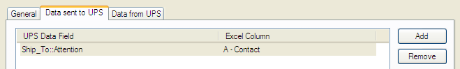
D. Now that the UPS Data Field and Excel Column are associated, OzLINK knows that the contact person being shipped to is listed in column A of your spreadsheet. You could also say that the 'Attention' section of the address is mapped to column A. Your setup screen should now match the picture below.
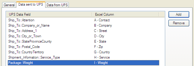
E. Now we'll map the rest of the information that is being sent to UPS. Complete steps A through D above for the following columns in your Excel spreadsheet: Company, Street, City, State, Zip, Country, Service, and Weight. Refer to the picture below for the exact 'UPS Data Field' names that you should use for each Excel Column.
6. Map the information you're getting back from UPS
Now we'll work on telling OzLINK which columns should be used to store the information that UPS will be sending back to us. Mapping these columns is very similar to the mapping from step 5.
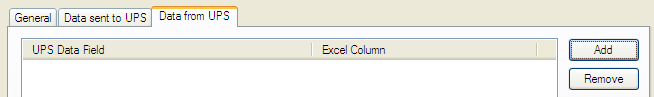
A. Click on the Data from UPS tab. Right now there is nothing in the list - we'll be adding an entry for each Excel column that will be receiving information.
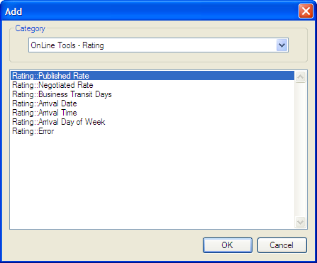
B. Click the Add button to add a new entry. The first column in our Excel sheet that will be receiving information is going to hold the UPS Published Rate. In the category dropdown, choose OnLine Tools - Rating. Select Rating::Published Rate, then click OK.
NOTE: For more details about what information is returned by each type of transaction, see:
Batch Data Returned.
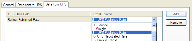
C. Rating::Published Rate will now be listed in the UPS Data Field section of the window. Next to it, in the Excel Column, click on the dropdown list and choose J - UPS Published Rate.
NOTE: If your Excel Column dropdown list only shows the column letters without the names, you can fix it by clicking OK, selecting a cell in your header row, and then returning to this screen by clicking Setup in the OzLINK toolbar, then the Data sent to UPS tab. The Excel Column dropdown list actually displays whatever is in the currently selected row, so selecting the header row while doing this setup is generally the easiest method.
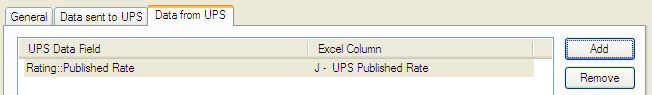
D. Now that the UPS Data Field and Excel Column are associated, OzLINK knows to put the published rate into column J when it gets information back from UPS. You could also say that the 'Published Rate' return information is mapped to column J. Your setup screen should now match the picture below.
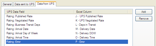
E. Now we'll map the rest of the information that is being received from UPS. Complete steps A through D above for the following columns in your Excel spreadsheet: UPS Negotiated Rate, Days in Transit, Delivery Date, Delivery DOW, Delivery Time, and Error. Refer to the picture below for the exact 'UPS Data Field' names that you should use for each Excel Column. Click OK when you're finished.
NOTE: You should always record the error in case anything goes wrong. The details noted in the error will help you to resolve any issues. There is a separate Error data field for each type of transaction, so be sure to select the one for rating.
6. Test your style
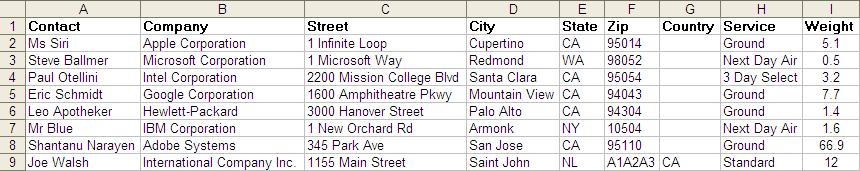
A. Now we'll need to enter some information in the spreadsheet so we can test out our style. Enter a few of the lines below, or copy them from the provided sample rating spreadsheet. (If you haven't seen it yet, you can
try the sample)
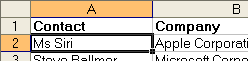
B. Select the Ms Siri cell by clicking on it. We do this because once we click the UPS button, OzLINK will process information from the currently selected row and move down from there.
C. Click on the Send to UPS button, then wait for processing to finish.
Microsoft Office 2003 or earlier:
The button will be in your main toolbar, and looks like this:
Microsoft Office 2007 or later:
Click on the Add-Ins tab to find the buttons added by OzLINK:
D. Clicking or typing will interrupt the process, so make sure the last line is finished before doing anything else.
E. You can now view the results in your Excel sheet. Your results will not match those below, but the cells will be filled in with rating information for each of the packages in your spreadsheet. You can use that information to make decisions about your shipments.
7. Use your New Style
Now that your style has been set up and tested, you can start entering your own information for real shipments. If you would like to create more styles or learn more about the options available, please use this tutorial as a guide and see any of the following.
Related Pages